Overview
iDEA: Integrative Differential expression and gene set Enrichment Analysis using summary statistics for single cell RNAseq studies
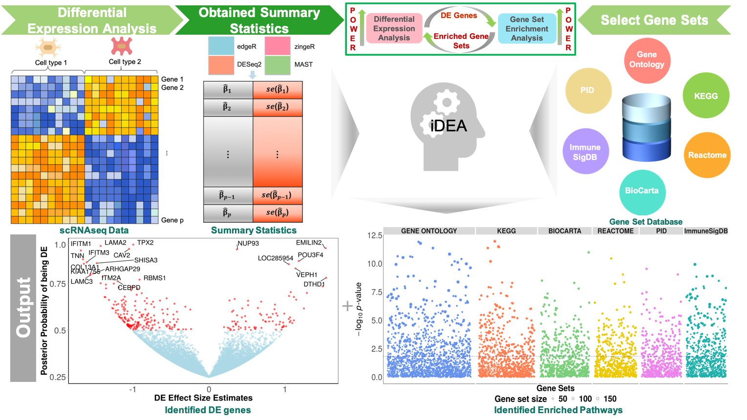
We developed a new computational method, iDEA, that enables powerful DE and GSE analysis for scRNAseq studies through integrative statistical modeling. Our method builds upon a hierarchical Bayesian model for joint modeling of DE and GSE analyses. It uses only summary statistics as input, allowing for effective data modeling through complementing and pairing with various existing DE methods. It relies on an efficient expectation-maximization algorithm with internal Markov Chain Monte Carlo steps for scalable inference. By integrating DE and GSE analyses, iDEA can improve the power and consistency of DE analysis and the accuracy of GSE analysis over common existing approaches. iDEA is implemented as an R package with source code freely available at: www.xzlab.org/software.html.
Required input data
iDEA requires two types of input data:
- gene-level summary statistics in terms of fold change/effect size estimates and their variances as inputs, which can be obtained using any existing single-cell RNAseq DE approaches (i.e., zingeR, MAST, etc.).
- Corresponding gene specific annotations, which are from the public databases (i.e., KEGG, Reactome, etc.). With DE test statistics as inputs, iDEA builds upon a hierarchical Bayesian model for joint modeling of GSEA and DE analysis.
1. Summary statistics, e.g.,
          beta   beta_var
A1BG     -1.028331e-02 0.005304736
A1BG-AS1 -2.173872e-03 0.008438381
A2M       8.671972e-06 0.002353646
...
The summary statistics file should be in data.frame data format with gene name as row names, while the column names are not required but the order of the column matters: the first column should be the coefficient and the second column should be the variance of the coefficient for each gene.
Here is an example of calculating standard error when you only have the p-value and beta coefficient available
## Assume you have obtained the DE results from i.e. zingeR, edgeR or MAST with the data frame res_DE (column: pvalue and LogFC)
pvalue <- res_DE$pvalue #### the pvalue column
zscore <- qnorm(pvalue/2.0, lower.tail=FALSE) #### convert the pvalue to z-score
beta <- res_DE$LogFC ## effect size
se_beta <- abs(beta/zscore) ## to approximate the standard error of beta
beta_var = se_beta^2  ### square
summary = data.frame(beta = beta,beta_var = beta_var)
## add the gene names as the rownames of summary
rownames(summary) = rownames(res_DE) ### or the gene id column in the res_DE results
2. Gene specific annotations, e.g.,
         annot1 annot2
A1BG     0      1
A1BG-AS1 1      0
A2M      0      0
...
The gene specific annotation file is required data.frame data format with gene name as row names, while the header is the gene specific annotation name. The row names of annotation file should match exactly with row names of summary statistics and should be in the same type, i.e. gene symbol or transcription id etc. If not, one solution is to use biomaRt R package to convert the gene name to make sure they are consistent each other.
We have provided both human gene sets and mouse gene sets in our package. Specifically, for human gene sets, we compiled seven exsiting gene set/pathway databases annotated on the reference genome GRCh37 from MSigDB databases (http://software.broadinstitute.org/gsea/downloads.jsp). These databases include BioCarta, KEGG, GO, PubChem Compound, ImmuneSigDB, PID and Reactome. For mouse gene sets, we downloaded the gene ontology (GO) annotations of mouse genes in the GAF 2.0 format from the website (http://www.informatics.jax.org/downloads/reports/index.html#go).
These human gene sets and mouse gene sets can be loaded from our package, i.e
data(humanGeneSets)
humanGeneSets[1:3,1:3]
       NAKAMURA_CANCER_MICROENVIRONMENT_UP NAKAMURA_CANCER_MICROENVIRONMENT_DN
MEF2C                                    0                                   0
ATP1B1                                   0                                   0
RORA                                     0                                   0
       WEST_ADRENOCORTICAL_TUMOR_MARKERS_UP
MEF2C                                     0
ATP1B1                                    0
RORA                                      0

data(mouseGeneSets)
mouseGeneSets[1:3,1:3]
           GO:0000002 GO:0000003 GO:0000009
MGI:101757          0          0          0
MGI:101758          0          0          0
MGI:101759          0          0          0
The organized gene sets can also be downloaded here for human gene sets, and here for mouse gene sets.
Getting started
library(iDEA)
1. Load summary statistics and annotations
In this tutorial, we will apply iDEA on a sample data from human embryonic stem cell from Chu et al to detect DE genes and enriched pathways. The summary statistics of DE analysis has been prepared by zingeR-DESeq2 method.
The example data can also be downloaded here for annotations, and here for summary statistics.
Load summary data,
data(summary_data)
head(summary_data)
##         log2FoldChange      lfcSE2
## A1BG      0.90779290 0.25796491
## A1CF      0.36390514 0.03568627
## A2LD1     0.03688353 0.75242959
## A2M       8.54034957 0.40550678
## A2ML1    -1.89816441 0.07381843
## AAAS      0.19593275 0.15456908
Load annotation data,
data(annotation_data)
head(annotation_data[,1:3])
##           GO_CELLULAR_RESPONSE_TO_LIPID GO_SECRETION_BY_CELL
## A1BG                              0                    1
## A1CF                              0                    0
## A2LD1                             0                    0
## A2M                               0                    1
## A2ML1                             0                    0
## AAAS                              0                    0
##       GO_REGULATION_OF_CANONICAL_WNT_SIGNALING_PATHWAY
## A1BG                                                 0
## A1CF                                                 0
## A2LD1                                                0
## A2M                                                  0
## A2ML1                                                0
## AAAS                                                 0
2. Create an iDEA object
We encourage the user set num_core > 1 if a large number of annotations is as input (Linux platform; for Windows platform, the num_core will be set 1, automatically).
The iDEA object is created by the function CreateiDEAObject. The essential inputs are:
- summary: summary statistics from common DE analsyis,with gene name as row names, while the first column should be the coefficient and the second column should be the variance of the coefficient for each gene. Data.frame foramt
- annotation: gene specific annotations, i.e gene sets from predefined database. The rownames should be matched with the summary statistics. Data.frame format.
- project: Default is “iDEA”.
- max_var_beta: the cutoff of the variance of the coefficient of genes. Genes with variance smaller than ‘max_var_beta’ are maintained. Default is 100
- min_percent_annot: the threshold of coverage rate (CR), i.e., the number of annotated genes (gene set size) divided by the number of tested genes. Default value is 0.0025.
- num_core: number of cores for parallel implementation. Default is 10.
idea <- CreateiDEAObject(summary_data, annotation_data, max_var_beta = 100, min_precent_annot = 0.0025, num_core=10)
The data are stored in idea@summary and idea@annotation.
head(idea@summary)
##           beta      beta_var
## A1BG      0.90779290 0.25796491
## A1CF      0.36390514 0.03568627
## A2LD1     0.03688353 0.75242959
## A2M       8.54034957 0.40550678
## A2ML1    -1.89816441 0.07381843
## AAAS      0.19593275 0.15456908
head(idea@annotation[[1]])
## 7 23 36 58 70 80
The gene indices which are annotated as 1 in the first gene set GO_CELLULAR_RESPONSE_TO_LIPID in our example annotation_data.
3. Fit the model
iDEA relies on an expectation-maximization (EM) algorithm with internal Markov chain Monte Carlo (MCMC) steps for scalable model inference.
The function iDEA.fit fits the iDEA model on the input data. The essential inputs are:
- object: iDEA object created by CreateiDEAObject.
- fit_noGS: boolean variable to indicate whether fitting the model without the annoation/gene set. Default is FALSE.
- init_beta: initial value for gene effect size, beta in MCMC sampling procedure. Default is NULL.
- init_tau: initial value for the coefficient of annotations/gene sets, including the intercept in EM procedure, default is c(-2,0.5).
- min_degene: the threshold for the number of detected DE genes in summary statistics. For some of extremely cases, the method does not work stably when the number of detected DE genes is 0.
- em_iter: maximum iteration for EM algorithm, default is 15
- mcmc_iter: maximum iteration for MCMC algorithm, default is 1000
- fit.tol: tolerance for fitting the model, default is 1e-5.
- verbose: print the messages about the fitting progresses. Default is TRUE.
- modelVariant: model option to run, boolean variable, if FALSE, runing the main iDEA model, which models on z score statistics. if TRUE, runing iDEA variant model which models on beta effect size.
idea <- iDEA.fit(idea,
                 fit_noGS=FALSE,
	         init_beta=NULL,
	         init_tau=c(-2,0.5),
	         min_degene=5,
	         em_iter=15,
	         mcmc_iter=1000,
	         fit.tol=1e-5,
                 modelVariant = F,
	         verbose=TRUE)
## ===== iDEA INPUT SUMMARY ==== ##
## number of annotations:  100
## number of genes:  15280
## number of cores:  10
## fitting the model with gene sets information...
  |======================================                                       |  50%, ETA 6:30
The results are stored in idea@de.
4. Correct p-values
iDEA utilizes Louis method to compute calibrated p-values for testing gene set enrichment, while simultaneously producing powerful posterior probability estimates for each gene being DE. The results are stored in idea@gsea.
idea <- iDEA.louis(idea) ##
|====================================== | 50%
5. Output from iDEA
GSE results from iDEA: the output of GSE results is stored in idea@gsea, with each row represents the gene set we tested.
head(idea@gsea)
                                          annot_id annot_coef  annot_var
1                    GO_CELLULAR_RESPONSE_TO_LIPID  0.3101074 0.01092405
2                             GO_SECRETION_BY_CELL  0.4803171 0.01033267
3 GO_REGULATION_OF_CANONICAL_WNT_SIGNALING_PATHWAY  0.3335924 0.01845976
4            GO_REGULATION_OF_DEVELOPMENTAL_GROWTH  0.7983761 0.01722159
5        GO_CELLULAR_RESPONSE_TO_EXTERNAL_STIMULUS  0.3097789 0.01745458
6                  GO_ACTIN_FILAMENT_BASED_PROCESS  0.7720139 0.01046010
  annot_var_louis sigma2_b pvalue_louis       pvalue
1      0.01548977 37.37384 1.271457e-02 3.007027e-03
2      0.01467251 37.38621 7.330424e-05 2.298691e-06
3      0.02674372 37.32392 4.136199e-02 1.407704e-02
4      0.02497394 37.35476 4.371900e-07 1.174085e-09
5      0.02448467 37.36763 4.773453e-02 1.903970e-02
6      0.01482588 37.42016 2.292072e-10 4.405020e-14
Specifically, the “annot_id” represents the gene set name, “annot_coef” is the estimated gene set enrichment parameter that determines the odds ratio of DE for genes inside the gene set versus genes outside the gene set. “annot_var” is the estimated variance of the annot_coef, “annot_var_louis” is the adjuested variance of the annot_coef by the Louis Method, “sigma2_b” is the scaling parameter. “pvalue_louis” is the pvalue calculated when applying Louis method to calibrate the pvalues while “pvalue” is the common pvalue without Louis Method correction.
DE results from iDEA: iDEA analyzes one gene set at a time, and perform the integrative differential expression analysis and gene set enrichment analysis. We can look at the DE results when adding the pre-selected gene set based on biological knowledge e.g.GO_REGULATION_OF_CANONICAL_WNT_SIGNALING_PATHWAY
### gene set coefficient estimate, tau_1 is the intercept, and tau_2 is the coefficient
idea@de[["GO_REGULATION_OF_CANONICAL_WNT_SIGNALING_PATHWAY"]]$annot_coef
      annot_coef
tau_1 -0.3567912
tau_2  0.3335924

### posterior inclusion probability of a gene being DE gene.
pip = unlist(idea@de[["GO_REGULATION_OF_CANONICAL_WNT_SIGNALING_PATHWAY"]]$pip)
### head the posterior inclusion probability for each gene
head(pip)
        PIP
A1BG  0.210
A1CF  0.120
A2LD1 0.105
A2M   1.000
A2ML1 1.000
AAAS  0.040
Certainly, sometimes it may not be easy to identify such pre-selected gene set for certain data sets. In the absence of pre-selected gene set, we developed a Bayesian model averaging (BMA) approach to aggregate DE evidence for any given genes across all available gene sets without the requirement of pre-selecting a gene set. See 6. Bayesian model averaging (BMA) approach.
6. Bayesian model averaging (BMA)
Here, we looked at the posterior inclusion probability (PIPs) for each gene infered by Bayesian model averaging (BMA) approach.
idea <- iDEA.BMA(idea) ##
head(idea@BMA_pip)
         BMA_pip
A1BG  0.21521492
A1CF  0.11058475
A2LD1 0.09177833
A2M   1.00000000
A2ML1 1.00000000
AAAS  0.04465690
The BMA approach yields consistent results for the majority of genes as compared to the pre-selection approach.
7. iDEA variant model
iDEA is mainly focusing on modeling the marginal effect size estimates and standard errors from DE analysis, which is equivalent to modeling of marginal z-scores. We also provide a variant of iDEA which models the cofficient of gene directly.
idea_variant <- iDEA.fit(idea,modelVariant = T) ##
|======================================                                       |  50%, ETA 6:47
idea_variant <- iDEA.louis(idea_variant)
|======================================                                       | 50%
###
The results format of using iDEA variant model and iDEA are the same.
8. Estimating FDR
Here we provide a method to calculate calibrated FDR estimates of gene sets based on permuted null distribution. Here we only permuted 10 times for the first 10 gene sets in annotation_data as an example to show the usage of iDEA on permutation. Basically, we construct an empirical null p-value distribution by permuting the gene labels for each gene set. This may take a long time, we recommend use more cores to run the permutation. The function iDEA.fit.null fits iDEA model by permuting gene labels in gene set, thus constructing tbe permuted null distribution for gene sets.
idea.null <- CreateiDEAObject(summary_data, annotation_data[,c(1:10)], num_core=10)
idea.null <- iDEA.fit.null(idea.null,numPermute = 10) ##
idea.null <- iDEA.louis(idea.null)
head(idea.null@gsea)
Then we have the pvalues under the permuted null, we can calculate FDR by using the function iDEA.FDR. The function iDEA.FDR calculate the estimated FDR for each gene set given the permuted null distribution of pvalues for gene sets. The inputs are:
- object.alt: iDEA object when runing iDEA on real gene sets.
- object.null: iDEA object when runing iDEA on permuted gene sets.
- numPermute: number of permutations used in idea.null. Default is 10. The results are returned as a data frame with FDR values estimated for each gene set.
df.FDR <- iDEA.FDR(idea,idea.null,numPermute = 10)
head(df.FDR)